
Computers are generally programmed to do what the developer dictates and will only behave predictably under the specified scenarios.
In recent years, people are increasingly turning to computers to perform tasks that can’t be achieved with traditional programming, which previously had to be done by humans performing manual tasks. Machine Learning gives computers the ability to “learn” and act on information based on observations without being explicitly programmed.
TechConnect entered the recent Get 2 the Core challenge on Unearthed’s crowd sourcing platform. This is TechConnect’s story, as part of the crowd sourcing approach, and does not imply or assert in any way that Newcrest Mining endorse Amazon Web Services or the work TechConnect have performed in this challenge.
Business problem
Currently a team at Newcrest Mining manually crop photographs of drill core samples before the photos can be fed into a system which detects the material type. This is extremely time-consuming due to the large number of photos. Hence why Newcrest Mining used crowd sourcing via the Unearthed platform, a platform bringing data scientists, start-ups and the energy & natural resources industry together.
Being able to automatically identify bounding box co-ordinates of the samples within an image would save 80-90% of the time spent preparing the photos.
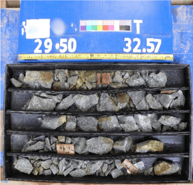
Input Image
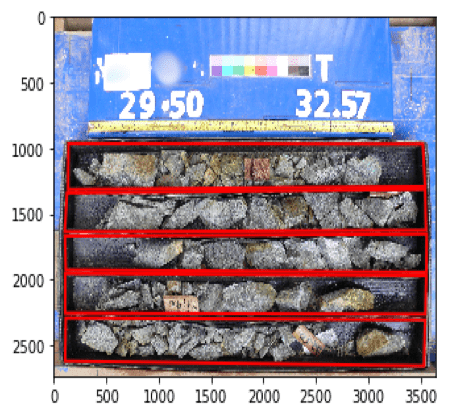
Expected Output Image
Before we can begin implementing an object-detection process, we first need to address a variety of issues with the photographs themselves, being:
- Not all photos are straight
- Not all core trays are in a fixed position relative to the camera
- Not all photos are taken perpendicular to the core trays introducing a perspective distortion
- Not all photos are high-resolution
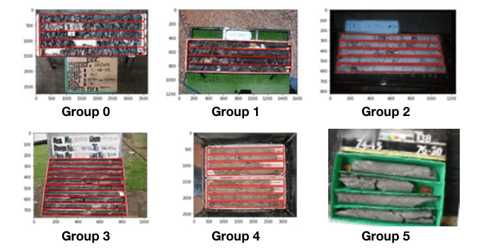
In addition to the object-classification, we need to use an image-classification process to classify each image into a group based on the factors above. The groups are defined as:
Group 0 – Core trays are positioned correctly in the images with no distortion. This is the ideal case
Group 1 – Core trays are misaligned in the image
Group 2 – Core trays have perspective distortion
Group 3 – Core trays are misaligned and have perspective distortion
Group 4 – The photo has a low aspect ratio
Group 5 – The photo has a low aspect ratio and are misaligned
Solution
We tried to solve this problem using Machine Learning. In particular, we used supervised learning. When conducting supervised learning the system is provided with the input data and the classification/label desired output for each data point. The system learns a model that when provided a previously seen input will reliably output the correct labelling or the most likely label when an unseen input is provided.
This differs from unsupervised learning. When utilising unsupervised techniques, the target label is unknown and the system must group or derive the label from the inherent properties within the data set itself.
The Supervised Machine Learning process works by:
- Obtaining, preparing & labelling the input data
- Create a model
- Train the model
- Test the model
- Deploy & use the model
There are many specific algorithms for supervised learning that are appropriate for different learning tasks. The object detection and classification problem of identifying core samples in images is particularly suited to a technique known as convolutional neural networks. The model “learns” by assigning and constantly adjusting internal weights and biases for each input of the training data to produce the specified output. The weights and biases become more accurate with more training data.
Amazon SageMaker provides a hosted platform that enabled us to quickly build, train, test and deploy our model.
Newcrest Mining provided a large collection of their photographs which contain core samples. A large subset of the photos also contained the expected output, which we used to train our model.
The expected output is a set of four (X, Y) coordinates per core sample in the photograph. The coordinates represent the corners of the bounding box that surrounds the core sample. Multiple sets of coordinates are expected for photos that contain multiple core samples.
The Process
We uploaded the supplied data to an AWS S3 bucket, using a separate prefix to separate images which we were provided the expected output for, and those with no output. S3 is an ideal store for the raw images with high durability, infinite capacity and direct integration with many other AWS products.
We further randomly split the photos with the expected output into a training dataset (70%) and a testing dataset (30%).
We created a Jupyter notebook on an Amazon SageMaker notebook instance to host and execute our code. By default the Jupyter notebook instance provides access to a wide variety of common data science tools such as numpy, tensorflow and matplotlib in addition to the Amazon SageMaker and AWS python SDKs. This allowed us to immediately focus on our particular problem of creating SageMaker compatible datasets with which we could build and test our models.
We trained our model by feeding the training dataset along with the expected output into an existing Sagemaker built object detection model to fine tune it to our specific problem. SageMaker has a collection of hyperparameters which influence how the model “learns”. Adjusting the hyperparameter values affects the overall accuracy of the model and how long the training takes. As the training proceeded we were able to monitor the changes to the primary accuracy metric and pre-emptively cancel any training configurations that did not perform well. This saved us considerable time and money by allowing us to abort poor configurations early.
We then tested the accuracy of our model by feeding testing data (data it has never see) without the output, then comparing the model’s output to the expected output.
After the first round of training we had our benchmark for accuracy. From there we were able to tune the model by iteratively adjusting the hyperparameters, model parameters and by augmenting the data set with additional examples then retraining and retesting. Setting the hyperparameter values is more of an artform than a science trial and error is often the best way.
We used a technique which dynamically assigned values to the learning rate after each epoch, similar to a harmonic progression:
This technique allowed us to start with large values to allow the model to converge quickly initially, then reduce the learning rate value by an increasingly smaller amount after each epoch as the model gets closer to an optimal solution. After many iterations of tuning, training and testing we had improved the overall accuracy of the model compared with our benchmark, and with our project deadline fast approaching we decided that it was accurate as possible in the timeframe that we had.
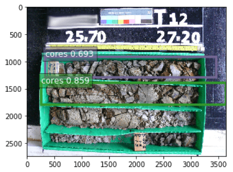
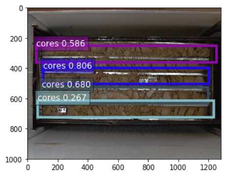
We then used our model to classify and detect the objects in the remaining photographs that didn’t exist in the training set. The following images show the bounding boxes around the cores that our model predicted:
Lessons Learned
Before we began we had an extremely high expectation of how accurate our model would be. In reality it wasn’t as accurate as our expectations.
We discussed things that could have made the model more accurate, train faster or both, including:
- Tuning the hyperparameters using SageMakers automated hyperparameter tuning tooling
- Copying the data across multiple regions to gain better access to the specific machine types we required for training
- Increasing the size of the training dataset by:
- Requesting more photographs
- Duplicating the provided photographs and modifying them slightly. This included:
- including duplicate copies of images and labels
- including copies after converting the images to greyscale
- including copies after changing the aspect ratio of the images
- including copies after mirroring the images
- Splitting the problem into separate, simpler machine learnable stages
- Strategies for identifying the corners of the cores when they are not a rectangle in the image
During these discussions we realised we hadn’t defined a cut-off for when we would consider our model to be “accurate enough”.
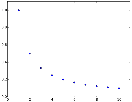
As a general rule the accuracy of the models you build improve most rapidly in the first few iterations, after that the rate of improvement slows significantly. Each subsequent improvement requires lengthier training, more sophisticated algorithms and models, more sophisticated feature engineering or substantial changes to approach entirely. This trend is depicted in the following chart:
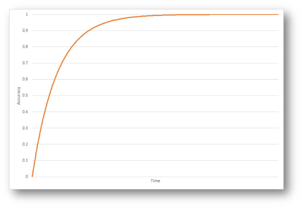
Depending on the use case, a model with an accuracy of 90% often requires significantly less training time, engineering effort and sophistication than a model with an accuracy of 93%. The acceptance criteria for a model needs to carefully balance these considerations to maximise the overall return on investment for the project.
In our case time was the factor that dictated when we stopped training and started using the model to produce the outputs for unseen photographs.
Thank you to the team at TechConnect that volunteered to try Amazon Sagemaker to address the Get 2 the Core Challenge posted by Newcrest Mining on the Unearthered portal. Also big thanks for sharing lessons learned and putting this blog together!